Evaluating water mass transformations from finite-volume tracer budget terms

Import packages

import warnings
import numpy as np
from dask.diagnostics import ProgressBar
import xarray as xr
import xhistogram
import xgcm
from xgcm import Grid
import matplotlib.pyplot as plt

print(
    'numpy version', np.__version__,
    '\nxarray version', xr.__version__,
    '\nxhistogram version', xhistogram.__version__,
    '\nxgcm version', xgcm.__version__
)

numpy version 2.4.2
xarray version 2026.2.0
xhistogram version 0.3.2
xgcm version 0.9.0

import xwmt
print('xwmt version', xwmt.__version__)

xwmt version 0.2.0

Load datasets and create strucutred grid object

The basic input for xwmt is an xgcm.Grid object that describes the structure of the underlying ocean model grid. To streamline this example, we use the helper function load_MOM6_coarsened_diagnostics to load the data and create the grid object. In later examples, we demonstrate how to build these objects from scratch.

from load_example_model_grid import load_MOM6_coarsened_diagnostics
grid = load_MOM6_coarsened_diagnostics()
display(grid)

File 'MOM6_global_example_sigma2_budgets_v0_0_6.nc' already exists at ../data/MOM6_global_example_sigma2_budgets_v0_0_6.nc. Skipping download.

<xgcm.Grid>
X Axis (periodic, boundary='periodic'):
  * center   xh --> outer
  * outer    xq --> center
Y Axis (not periodic, boundary='extend'):
  * center   yh --> outer
  * outer    yq --> center
Z Axis (not periodic, boundary='extend'):
  * center   sigma2_l --> outer
  * outer    sigma2_i --> center

Note: In addition to grid containing information about the static model grid, its attribute grid._ds points to the full dataset containing model diagnostics!

display(grid._ds)

<xarray.Dataset> Size: 1GB
Dimensions:                         (time_bounds: 2, sigma2_l: 74, yh: 180,
                                     xh: 240, time: 1, xq: 241, yq: 181,
                                     sigma2_i: 75)
Coordinates: (12/28)
  * time_bounds                     (time_bounds) object 16B 2000-01-01 00:00...
    time_bounds_since_init          (time_bounds) object 16B dask.array<chunksize=(2,), meta=np.ndarray>
  * sigma2_l                        (sigma2_l) float64 592B 4.246 ... 38.49
    rho2_l                          (sigma2_l) float64 592B dask.array<chunksize=(74,), meta=np.ndarray>
  * yh                              (yh) int64 1kB 0 1 2 3 4 ... 176 177 178 179
  * xh                              (xh) int64 2kB 0 1 2 3 4 ... 236 237 238 239
    ...                              ...
    geolon_c                        (yq, xq) float64 349kB dask.array<chunksize=(181, 241), meta=np.ndarray>
    geolon_u                        (yh, xq) float64 347kB dask.array<chunksize=(180, 241), meta=np.ndarray>
    wet_u                           (yh, xq) float32 174kB dask.array<chunksize=(180, 241), meta=np.ndarray>
  * yq                              (yq) int64 1kB 0 1 2 3 4 ... 177 178 179 180
  * sigma2_i                        (sigma2_i) float64 600B -3.0 11.49 ... 39.0
    rho2_i                          (sigma2_i) float64 600B dask.array<chunksize=(75,), meta=np.ndarray>
Data variables: (12/46)
    sigma2_bounds                   (time_bounds, sigma2_l, yh, xh) float64 51MB dask.array<chunksize=(2, 74, 180, 240), meta=np.ndarray>
    so_bounds                       (time_bounds, sigma2_l, yh, xh) float32 26MB dask.array<chunksize=(2, 74, 180, 240), meta=np.ndarray>
    thetao_bounds                   (time_bounds, sigma2_l, yh, xh) float32 26MB dask.array<chunksize=(2, 74, 180, 240), meta=np.ndarray>
    thkcello_bounds                 (time_bounds, sigma2_l, yh, xh) float32 26MB dask.array<chunksize=(2, 74, 180, 240), meta=np.ndarray>
    S_advection_xy                  (time, sigma2_l, yh, xh) float64 26MB dask.array<chunksize=(1, 74, 180, 240), meta=np.ndarray>
    Sh_tendency_vert_remap          (time, sigma2_l, yh, xh) float64 26MB dask.array<chunksize=(1, 74, 180, 240), meta=np.ndarray>
    ...                              ...
    umo                             (time, sigma2_l, yh, xq) float64 26MB dask.array<chunksize=(1, 74, 180, 241), meta=np.ndarray>
    vert_remap_h_tendency           (time, sigma2_l, yh, xh) float64 26MB dask.array<chunksize=(1, 74, 180, 240), meta=np.ndarray>
    vmo                             (time, sigma2_l, yq, xh) float64 26MB dask.array<chunksize=(1, 74, 181, 240), meta=np.ndarray>
    vprec                           (time, sigma2_l, yh, xh) float64 26MB dask.array<chunksize=(1, 74, 180, 240), meta=np.ndarray>
    wfo                             (time, sigma2_l, yh, xh) float64 26MB dask.array<chunksize=(1, 74, 180, 240), meta=np.ndarray>
    zos                             (time, yh, xh) float64 346kB dask.array<chunksize=(1, 180, 240), meta=np.ndarray>
Attributes:
    description:  An example netcdf file containing all variables required to...
    version:      0_0_6
    doi:          10.5281/zenodo.15384910

xarray.Dataset

• Dimensions:
  • time_bounds: 2
  • sigma2_l: 74
  • yh: 180
  • xh: 240
  • time: 1
  • xq: 241
  • yq: 181
  • sigma2_i: 75
• Coordinates: (28)
  • time_bounds
    (time_bounds)
    object
    2000-01-01 00:00:00 2001-01-01 0...

    axis :

    T

    calendar_type :

    NOLEAP

    cell_methods :

    time:point

    long_name :

    historical time

    array([cftime.DatetimeNoLeap(2000, 1, 1, 0, 0, 0, 0, has_year_zero=True),
           cftime.DatetimeNoLeap(2001, 1, 1, 0, 0, 0, 0, has_year_zero=True)],
          dtype=object)

  • time_bounds_since_init
    (time_bounds)
    object
    dask.array<chunksize=(2,), meta=np.ndarray>

    axis :

    T

    calendar_type :

    NOLEAP

    cell_methods :

    time:point

    long_name :

    time since model initialization

    Array Chunk Bytes 16 B 16 B Shape (2,) (2,) Dask graph 1 chunks in 2 graph layers Data type object numpy.ndarray

  • sigma2_l
    (sigma2_l)
    float64
    4.246 13.57 17.71 ... 37.9 38.49

    axis :

    Z

    cell_methods :

    sigma2_l:point

    edges :

    sigma2_i

    long_name :

    Target Potential Density minus 1000 kg/m3 at cell center

    positive :

    down

    units :

    kg m-3

    array([ 4.24625, 13.565  , 17.71   , 21.855  , 25.96375, 28.165  , 28.495  ,
           28.83   , 29.165  , 29.495  , 29.83   , 30.165  , 30.495  , 30.83   ,
           31.165  , 31.495  , 31.83   , 32.165  , 32.495  , 32.83   , 33.0665 ,
           33.28225, 33.571  , 33.8425 , 34.09975, 34.3435 , 34.5735 , 34.7895 ,
           34.991  , 35.17725, 35.348  , 35.5035 , 35.64475, 35.77275, 35.8885 ,
           35.99375, 36.09025, 36.17925, 36.262  , 36.34   , 36.4145 , 36.4865 ,
           36.5565 , 36.625  , 36.692  , 36.75525, 36.812  , 36.86125, 36.904  ,
           36.9415 , 36.974  , 37.002  , 37.02625, 37.0475 , 37.0665 , 37.08375,
           37.1    , 37.116  , 37.132  , 37.148  , 37.164  , 37.18   , 37.1965 ,
           37.2145 , 37.235  , 37.26   , 37.2945 , 37.345  , 37.415  , 37.5075 ,
           37.625  , 37.76   , 37.9    , 38.485  ])

  • rho2_l
    (sigma2_l)
    float64
    dask.array<chunksize=(74,), meta=np.ndarray>

    axis :

    Z

    edges :

    rho2_i

    long_name :

    Target Potential Density at cell center

    positive :

    down

    units :

    kg m-3

    Array Chunk Bytes 592 B 592 B Shape (74,) (74,) Dask graph 1 chunks in 2 graph layers Data type float64 numpy.ndarray

  • yh
    (yh)
    int64
    0 1 2 3 4 5 ... 175 176 177 178 179

    cell_methods :

    yh:point

    long_name :

    cell center y-index (nominally latitude)

    array([  0,   1,   2,   3,   4,   5,   6,   7,   8,   9,  10,  11,  12,  13,
            14,  15,  16,  17,  18,  19,  20,  21,  22,  23,  24,  25,  26,  27,
            28,  29,  30,  31,  32,  33,  34,  35,  36,  37,  38,  39,  40,  41,
            42,  43,  44,  45,  46,  47,  48,  49,  50,  51,  52,  53,  54,  55,
            56,  57,  58,  59,  60,  61,  62,  63,  64,  65,  66,  67,  68,  69,
            70,  71,  72,  73,  74,  75,  76,  77,  78,  79,  80,  81,  82,  83,
            84,  85,  86,  87,  88,  89,  90,  91,  92,  93,  94,  95,  96,  97,
            98,  99, 100, 101, 102, 103, 104, 105, 106, 107, 108, 109, 110, 111,
           112, 113, 114, 115, 116, 117, 118, 119, 120, 121, 122, 123, 124, 125,
           126, 127, 128, 129, 130, 131, 132, 133, 134, 135, 136, 137, 138, 139,
           140, 141, 142, 143, 144, 145, 146, 147, 148, 149, 150, 151, 152, 153,
           154, 155, 156, 157, 158, 159, 160, 161, 162, 163, 164, 165, 166, 167,
           168, 169, 170, 171, 172, 173, 174, 175, 176, 177, 178, 179])

  • xh
    (xh)
    int64
    0 1 2 3 4 5 ... 235 236 237 238 239

    cell_methods :

    xh:point

    long_name :

    cell center x-index (nominally longitude)

    array([  0,   1,   2, ..., 237, 238, 239], shape=(240,))

  • areacello
    (yh, xh)
    float64
    dask.array<chunksize=(180, 240), meta=np.ndarray>

    cell_methods :

    area:sum yh:sum xh:sum time: point

    long_name :

    Ocean Grid-Cell Area

    note :

    We ignore land cells in partially wet cells when coarsening, so that tracer content can be accurately reconstructed by multiplying coarsened area-averaged tendencies by it. Fully wet (`wet==1.0`) and fully dry (`wet==0.0`) cells should be unaffected, and will just represent the total cell area. For the partially wet cells, total cell area can be derived from the ocean area by divding `areacello` by `wet`.

    standard_name :

    cell_area

    units :

    m2

    Array Chunk Bytes 337.50 kiB 337.50 kiB Shape (180, 240) (180, 240) Dask graph 1 chunks in 2 graph layers Data type float64 numpy.ndarray

  • deptho
    (yh, xh)
    float32
    dask.array<chunksize=(180, 240), meta=np.ndarray>

    cell_measures :

    area: areacello

    cell_methods :

    xh:mean yh:mean time:point

    long_name :

    Sea Floor Depth

    standard_name :

    sea_floor_depth_below_geoid

    units :

    m

    Array Chunk Bytes 168.75 kiB 168.75 kiB Shape (180, 240) (180, 240) Dask graph 1 chunks in 2 graph layers Data type float32 numpy.ndarray

  • dxCv
    (yq, xh)
    float64
    dask.array<chunksize=(181, 240), meta=np.ndarray>

    cell_methods :

    xh:sum yq:point time:point

    interp_method :

    none

    long_name :

    Delta(x) at v points (meter)

    units :

    m

    Array Chunk Bytes 339.38 kiB 339.38 kiB Shape (181, 240) (181, 240) Dask graph 1 chunks in 2 graph layers Data type float64 numpy.ndarray

  • geolat
    (yh, xh)
    float64
    dask.array<chunksize=(180, 240), meta=np.ndarray>

    cell_methods :

    time: point

    long_name :

    Latitude of tracer (T) points

    units :

    degrees_north

    Array Chunk Bytes 337.50 kiB 337.50 kiB Shape (180, 240) (180, 240) Dask graph 1 chunks in 2 graph layers Data type float64 numpy.ndarray

  • geolat_v
    (yq, xh)
    float64
    dask.array<chunksize=(181, 240), meta=np.ndarray>

    cell_methods :

    time: point

    interp_method :

    none

    long_name :

    Latitude of meridional velocity (Cv) points

    units :

    degrees_north

    Array Chunk Bytes 339.38 kiB 339.38 kiB Shape (181, 240) (181, 240) Dask graph 1 chunks in 2 graph layers Data type float64 numpy.ndarray

  • geolon
    (yh, xh)
    float64
    dask.array<chunksize=(180, 240), meta=np.ndarray>

    cell_methods :

    time: point

    long_name :

    Longitude of tracer (T) points

    units :

    degrees_east

    Array Chunk Bytes 337.50 kiB 337.50 kiB Shape (180, 240) (180, 240) Dask graph 1 chunks in 2 graph layers Data type float64 numpy.ndarray

  • geolon_v
    (yq, xh)
    float64
    dask.array<chunksize=(181, 240), meta=np.ndarray>

    cell_methods :

    time: point

    interp_method :

    none

    long_name :

    Longitude of meridional velocity (Cv) points

    units :

    degrees_east

    Array Chunk Bytes 339.38 kiB 339.38 kiB Shape (181, 240) (181, 240) Dask graph 1 chunks in 2 graph layers Data type float64 numpy.ndarray

  • lat
    (yh, xh)
    float64
    dask.array<chunksize=(180, 240), meta=np.ndarray>

    cell_methods :

    time: point

    long_name :

    Latitude of tracer (T) points

    units :

    degrees_north

    Array Chunk Bytes 337.50 kiB 337.50 kiB Shape (180, 240) (180, 240) Dask graph 1 chunks in 2 graph layers Data type float64 numpy.ndarray

  • lon
    (yh, xh)
    float64
    dask.array<chunksize=(180, 240), meta=np.ndarray>

    cell_methods :

    time: point

    long_name :

    Longitude of tracer (T) points

    units :

    degrees_east

    Array Chunk Bytes 337.50 kiB 337.50 kiB Shape (180, 240) (180, 240) Dask graph 1 chunks in 2 graph layers Data type float64 numpy.ndarray

  • wet
    (yh, xh)
    float32
    dask.array<chunksize=(180, 240), meta=np.ndarray>

    cell_measures :

    area: areacello

    cell_methods :

    xh:mean yh:mean time:point

    long_name :

    0 if land, 1 if ocean at tracer points

    note :

    Can be between 0 and 1 if coarse cell includes both wet and dry sub-cells.

    Array Chunk Bytes 168.75 kiB 168.75 kiB Shape (180, 240) (180, 240) Dask graph 1 chunks in 2 graph layers Data type float32 numpy.ndarray

  • wet_v
    (yq, xh)
    float32
    dask.array<chunksize=(181, 240), meta=np.ndarray>

    cell_methods :

    xh:mean yq:point time:point

    interp_method :

    none

    long_name :

    0 if land, 1 if ocean at meridional velocity (Cv) points

    note :

    Can be between 0 and 1 if coarse face includes both wet and dry sub-faces.

    Array Chunk Bytes 169.69 kiB 169.69 kiB Shape (181, 240) (181, 240) Dask graph 1 chunks in 2 graph layers Data type float32 numpy.ndarray

  • time
    (time)
    object
    2000-07-01 00:00:00

    axis :

    T

    bounds :

    time_bnds

    calendar_type :

    NOLEAP

    cell_methods :

    time:mean

    long_name :

    historical time

    array([cftime.DatetimeNoLeap(2000, 7, 1, 0, 0, 0, 0, has_year_zero=True)],
          dtype=object)

  • xq
    (xq)
    int64
    0 1 2 3 4 5 ... 236 237 238 239 240

    cell_methods :

    xq:point

    long_name :

    cell corner x-index (nominally longitude)

    array([  0,   1,   2, ..., 238, 239, 240], shape=(241,))

  • dyCu
    (yh, xq)
    float64
    dask.array<chunksize=(180, 241), meta=np.ndarray>

    cell_methods :

    xq:point yh:sum time:point

    interp_method :

    none

    long_name :

    Delta(y) at u points (meter)

    units :

    m

    Array Chunk Bytes 338.91 kiB 338.91 kiB Shape (180, 241) (180, 241) Dask graph 1 chunks in 2 graph layers Data type float64 numpy.ndarray

  • geolat_c
    (yq, xq)
    float64
    dask.array<chunksize=(181, 241), meta=np.ndarray>

    cell_methods :

    time: point

    interp_method :

    none

    long_name :

    Latitude of corner (Bu) points

    units :

    degrees_north

    Array Chunk Bytes 340.79 kiB 340.79 kiB Shape (181, 241) (181, 241) Dask graph 1 chunks in 2 graph layers Data type float64 numpy.ndarray

  • geolat_u
    (yh, xq)
    float64
    dask.array<chunksize=(180, 241), meta=np.ndarray>

    cell_methods :

    time: point

    interp_method :

    none

    long_name :

    Latitude of zonal velocity (Cu) points

    units :

    degrees_north

    Array Chunk Bytes 338.91 kiB 338.91 kiB Shape (180, 241) (180, 241) Dask graph 1 chunks in 2 graph layers Data type float64 numpy.ndarray

  • geolon_c
    (yq, xq)
    float64
    dask.array<chunksize=(181, 241), meta=np.ndarray>

    cell_methods :

    time: point

    interp_method :

    none

    long_name :

    Longitude of corner (Bu) points

    units :

    degrees_east

    Array Chunk Bytes 340.79 kiB 340.79 kiB Shape (181, 241) (181, 241) Dask graph 1 chunks in 2 graph layers Data type float64 numpy.ndarray

  • geolon_u
    (yh, xq)
    float64
    dask.array<chunksize=(180, 241), meta=np.ndarray>

    cell_methods :

    time: point

    interp_method :

    none

    long_name :

    Longitude of zonal velocity (Cu) points

    units :

    degrees_east

    Array Chunk Bytes 338.91 kiB 338.91 kiB Shape (180, 241) (180, 241) Dask graph 1 chunks in 2 graph layers Data type float64 numpy.ndarray

  • wet_u
    (yh, xq)
    float32
    dask.array<chunksize=(180, 241), meta=np.ndarray>

    cell_methods :

    xq:point yh:mean time:point

    interp_method :

    none

    long_name :

    0 if land, 1 if ocean at zonal velocity (Cu) points

    note :

    Can be between 0 and 1 if coarse face includes both wet and dry sub-faces.

    Array Chunk Bytes 169.45 kiB 169.45 kiB Shape (180, 241) (180, 241) Dask graph 1 chunks in 2 graph layers Data type float32 numpy.ndarray

  • yq
    (yq)
    int64
    0 1 2 3 4 5 ... 176 177 178 179 180

    cell_methods :

    yq:point

    long_name :

    cell corner y-index (nominally latitude)

    array([  0,   1,   2,   3,   4,   5,   6,   7,   8,   9,  10,  11,  12,  13,
            14,  15,  16,  17,  18,  19,  20,  21,  22,  23,  24,  25,  26,  27,
            28,  29,  30,  31,  32,  33,  34,  35,  36,  37,  38,  39,  40,  41,
            42,  43,  44,  45,  46,  47,  48,  49,  50,  51,  52,  53,  54,  55,
            56,  57,  58,  59,  60,  61,  62,  63,  64,  65,  66,  67,  68,  69,
            70,  71,  72,  73,  74,  75,  76,  77,  78,  79,  80,  81,  82,  83,
            84,  85,  86,  87,  88,  89,  90,  91,  92,  93,  94,  95,  96,  97,
            98,  99, 100, 101, 102, 103, 104, 105, 106, 107, 108, 109, 110, 111,
           112, 113, 114, 115, 116, 117, 118, 119, 120, 121, 122, 123, 124, 125,
           126, 127, 128, 129, 130, 131, 132, 133, 134, 135, 136, 137, 138, 139,
           140, 141, 142, 143, 144, 145, 146, 147, 148, 149, 150, 151, 152, 153,
           154, 155, 156, 157, 158, 159, 160, 161, 162, 163, 164, 165, 166, 167,
           168, 169, 170, 171, 172, 173, 174, 175, 176, 177, 178, 179, 180])

  • sigma2_i
    (sigma2_i)
    float64
    -3.0 11.49 15.64 ... 37.97 39.0

    axis :

    Z

    cell_methods :

    sigma2_i:point

    long_name :

    Target Potential Density minus 1000 kg/m3 at interface

    positive :

    down

    units :

    kg m-3

    array([-3.    , 11.4925, 15.6375, 19.7825, 23.9275, 28.    , 28.33  , 28.66  ,
           29.    , 29.33  , 29.66  , 30.    , 30.33  , 30.66  , 31.    , 31.33  ,
           31.66  , 32.    , 32.33  , 32.66  , 33.    , 33.133 , 33.4315, 33.7105,
           33.9745, 34.225 , 34.462 , 34.685 , 34.894 , 35.088 , 35.2665, 35.4295,
           35.5775, 35.712 , 35.8335, 35.9435, 36.044 , 36.1365, 36.222 , 36.302 ,
           36.378 , 36.451 , 36.522 , 36.591 , 36.659 , 36.725 , 36.7855, 36.8385,
           36.884 , 36.924 , 36.959 , 36.989 , 37.015 , 37.0375, 37.0575, 37.0755,
           37.092 , 37.108 , 37.124 , 37.14  , 37.156 , 37.172 , 37.188 , 37.205 ,
           37.224 , 37.246 , 37.274 , 37.315 , 37.375 , 37.455 , 37.56  , 37.69  ,
           37.83  , 37.97  , 39.    ])

  • rho2_i
    (sigma2_i)
    float64
    dask.array<chunksize=(75,), meta=np.ndarray>

    axis :

    Z

    long_name :

    Target Potential Density at interface

    positive :

    down

    units :

    kg m-3

    Array Chunk Bytes 600 B 600 B Shape (75,) (75,) Dask graph 1 chunks in 2 graph layers Data type float64 numpy.ndarray

• Data variables: (46)
  • sigma2_bounds
    (time_bounds, sigma2_l, yh, xh)
    float64
    dask.array<chunksize=(2, 74, 180, 240), meta=np.ndarray>

    area :

    areacello

    cell_methods :

    area:mean sigma2_l:mean yh:mean xh:mean time:point

    description :

    Computed offline using the gsw python package implementation of TEOS10.

    long_name :

    Potential Density referenced to 2000 dbar (minus 1000 kg/m3)

    units :

    kg m-3

    volume :

    volcello

    Array Chunk Bytes 48.78 MiB 48.78 MiB Shape (2, 74, 180, 240) (2, 74, 180, 240) Dask graph 1 chunks in 5 graph layers Data type float64 numpy.ndarray

  • so_bounds
    (time_bounds, sigma2_l, yh, xh)
    float32
    dask.array<chunksize=(2, 74, 180, 240), meta=np.ndarray>

    cell_measures :

    volume: volcello area: areacello

    cell_methods :

    area:mean sigma2_l:mean yh:mean xh:mean time:point

    long_name :

    Sea Water Salinity

    standard_name :

    sea_water_salinity

    units :

    psu

    Array Chunk Bytes 24.39 MiB 24.39 MiB Shape (2, 74, 180, 240) (2, 74, 180, 240) Dask graph 1 chunks in 5 graph layers Data type float32 numpy.ndarray

  • thetao_bounds
    (time_bounds, sigma2_l, yh, xh)
    float32
    dask.array<chunksize=(2, 74, 180, 240), meta=np.ndarray>

    cell_measures :

    volume: volcello area: areacello

    cell_methods :

    area:mean sigma2_l:mean yh:mean xh:mean time:point

    long_name :

    Sea Water Potential Temperature

    standard_name :

    sea_water_potential_temperature

    units :

    degC

    Array Chunk Bytes 24.39 MiB 24.39 MiB Shape (2, 74, 180, 240) (2, 74, 180, 240) Dask graph 1 chunks in 5 graph layers Data type float32 numpy.ndarray

  • thkcello_bounds
    (time_bounds, sigma2_l, yh, xh)
    float32
    dask.array<chunksize=(2, 74, 180, 240), meta=np.ndarray>

    cell_measures :

    volume: volcello area: areacello

    cell_methods :

    area:mean sigma2_l:sum yh:mean xh:mean time:point

    long_name :

    Cell Thickness

    standard_name :

    cell_thickness

    units :

    m

    Array Chunk Bytes 24.39 MiB 24.39 MiB Shape (2, 74, 180, 240) (2, 74, 180, 240) Dask graph 1 chunks in 5 graph layers Data type float32 numpy.ndarray

  • S_advection_xy
    (time, sigma2_l, yh, xh)
    float64
    dask.array<chunksize=(1, 74, 180, 240), meta=np.ndarray>

    cell_measures :

    volume: volcello area: areacello

    cell_methods :

    area:mean sigma2_l:sum yh:mean xh:mean time:mean

    long_name :

    Horizontal convergence of residual mean advective fluxes of salt

    time_avg_info :

    average_T1,average_T2,average_DT

    units :

    kg m-2 s-1

    Array Chunk Bytes 24.39 MiB 24.39 MiB Shape (1, 74, 180, 240) (1, 74, 180, 240) Dask graph 1 chunks in 5 graph layers Data type float64 numpy.ndarray

  • Sh_tendency_vert_remap
    (time, sigma2_l, yh, xh)
    float64
    dask.array<chunksize=(1, 74, 180, 240), meta=np.ndarray>

    cell_measures :

    volume: volcello area: areacello

    cell_methods :

    area:mean sigma2_l:sum yh:mean xh:mean time:mean

    long_name :

    Vertical remapping tracer content tendency for Salt

    time_avg_info :

    average_T1,average_T2,average_DT

    units :

    kg m-2 s-1

    Array Chunk Bytes 24.39 MiB 24.39 MiB Shape (1, 74, 180, 240) (1, 74, 180, 240) Dask graph 1 chunks in 5 graph layers Data type float64 numpy.ndarray

  • T_advection_xy
    (time, sigma2_l, yh, xh)
    float64
    dask.array<chunksize=(1, 74, 180, 240), meta=np.ndarray>

    cell_measures :

    volume: volcello area: areacello

    cell_methods :

    area:mean sigma2_l:sum yh:mean xh:mean time:mean

    long_name :

    Horizontal convergence of residual mean advective fluxes of heat

    time_avg_info :

    average_T1,average_T2,average_DT

    units :

    W m-2

    Array Chunk Bytes 24.39 MiB 24.39 MiB Shape (1, 74, 180, 240) (1, 74, 180, 240) Dask graph 1 chunks in 5 graph layers Data type float64 numpy.ndarray

  • Th_tendency_vert_remap
    (time, sigma2_l, yh, xh)
    float64
    dask.array<chunksize=(1, 74, 180, 240), meta=np.ndarray>

    cell_measures :

    volume: volcello area: areacello

    cell_methods :

    area:mean sigma2_l:sum yh:mean xh:mean time:mean

    long_name :

    Vertical remapping tracer content tendency for Heat

    time_avg_info :

    average_T1,average_T2,average_DT

    units :

    W m-2

    Array Chunk Bytes 24.39 MiB 24.39 MiB Shape (1, 74, 180, 240) (1, 74, 180, 240) Dask graph 1 chunks in 5 graph layers Data type float64 numpy.ndarray

  • boundary_forcing_h_tendency
    (time, sigma2_l, yh, xh)
    float64
    dask.array<chunksize=(1, 74, 180, 240), meta=np.ndarray>

    cell_measures :

    volume: volcello area: areacello

    cell_methods :

    area:mean sigma2_l:sum yh:mean xh:mean time:mean

    long_name :

    Cell thickness tendency due to boundary forcing

    time_avg_info :

    average_T1,average_T2,average_DT

    units :

    m s-1

    Array Chunk Bytes 24.39 MiB 24.39 MiB Shape (1, 74, 180, 240) (1, 74, 180, 240) Dask graph 1 chunks in 5 graph layers Data type float64 numpy.ndarray

  • boundary_forcing_heat_tendency
    (time, sigma2_l, yh, xh)
    float64
    dask.array<chunksize=(1, 74, 180, 240), meta=np.ndarray>

    cell_measures :

    volume: volcello area: areacello

    cell_methods :

    area:mean sigma2_l:sum yh:mean xh:mean time:mean

    long_name :

    Boundary forcing heat tendency

    time_avg_info :

    average_T1,average_T2,average_DT

    units :

    W m-2

    Array Chunk Bytes 24.39 MiB 24.39 MiB Shape (1, 74, 180, 240) (1, 74, 180, 240) Dask graph 1 chunks in 5 graph layers Data type float64 numpy.ndarray

  • boundary_forcing_salt_tendency
    (time, sigma2_l, yh, xh)
    float64
    dask.array<chunksize=(1, 74, 180, 240), meta=np.ndarray>

    cell_measures :

    volume: volcello area: areacello

    cell_methods :

    area:mean sigma2_l:sum yh:mean xh:mean time:mean

    long_name :

    Boundary forcing salt tendency

    time_avg_info :

    average_T1,average_T2,average_DT

    units :

    kg m-2 s-1

    Array Chunk Bytes 24.39 MiB 24.39 MiB Shape (1, 74, 180, 240) (1, 74, 180, 240) Dask graph 1 chunks in 5 graph layers Data type float64 numpy.ndarray

  • dhdt
    (time, sigma2_l, yh, xh)
    float64
    dask.array<chunksize=(1, 74, 180, 240), meta=np.ndarray>

    cell_measures :

    volume: volcello area: areacello

    cell_methods :

    area:mean sigma2_l:sum yh:mean xh:mean time:mean

    long_name :

    Thickness tendency

    time_avg_info :

    average_T1,average_T2,average_DT

    units :

    m s-1

    Array Chunk Bytes 24.39 MiB 24.39 MiB Shape (1, 74, 180, 240) (1, 74, 180, 240) Dask graph 1 chunks in 5 graph layers Data type float64 numpy.ndarray

  • dynamics_h_tendency
    (time, sigma2_l, yh, xh)
    float64
    dask.array<chunksize=(1, 74, 180, 240), meta=np.ndarray>

    cell_measures :

    volume: volcello area: areacello

    cell_methods :

    area:mean sigma2_l:sum yh:mean xh:mean time:mean

    long_name :

    Change in layer thicknesses due to horizontal dynamics

    time_avg_info :

    average_T1,average_T2,average_DT

    units :

    m s-1

    Array Chunk Bytes 24.39 MiB 24.39 MiB Shape (1, 74, 180, 240) (1, 74, 180, 240) Dask graph 1 chunks in 5 graph layers Data type float64 numpy.ndarray

  • ePBL_h_ML
    (time, yh, xh)
    float64
    dask.array<chunksize=(1, 180, 240), meta=np.ndarray>

    cell_measures :

    area: areacello

    cell_methods :

    area:mean yh:mean xh:mean time: mean

    long_name :

    Surface boundary layer depth

    time_avg_info :

    average_T1,average_T2,average_DT

    units :

    m

    Array Chunk Bytes 337.50 kiB 337.50 kiB Shape (1, 180, 240) (1, 180, 240) Dask graph 1 chunks in 5 graph layers Data type float64 numpy.ndarray

  • evs
    (time, sigma2_l, yh, xh)
    float64
    dask.array<chunksize=(1, 74, 180, 240), meta=np.ndarray>

    cell_measures :

    area: areacello

    cell_methods :

    area:mean sigma2_l:sum yh:mean xh:mean time:mean

    long_name :

    Convergence of Water Evaporation Flux Where Ice Free Ocean over Sea

    standard_name :

    water_evaporation_flux

    time_avg_info :

    average_T1,average_T2,average_DT

    units :

    kg m-2 s-1

    Array Chunk Bytes 24.39 MiB 24.39 MiB Shape (1, 74, 180, 240) (1, 74, 180, 240) Dask graph 1 chunks in 5 graph layers Data type float64 numpy.ndarray

  • ficeberg
    (time, sigma2_l, yh, xh)
    float64
    dask.array<chunksize=(1, 74, 180, 240), meta=np.ndarray>

    cell_measures :

    area: areacello

    cell_methods :

    area:mean sigma2_l:sum yh:mean xh:mean time:mean

    long_name :

    Convergence of Water Flux into Seawater from Icebergs

    standard_name :

    water_flux_into_sea_water_from_icebergs

    time_avg_info :

    average_T1,average_T2,average_DT

    units :

    kg m-2 s-1

    Array Chunk Bytes 24.39 MiB 24.39 MiB Shape (1, 74, 180, 240) (1, 74, 180, 240) Dask graph 1 chunks in 5 graph layers Data type float64 numpy.ndarray

  • frazil_heat_tendency
    (time, sigma2_l, yh, xh)
    float64
    dask.array<chunksize=(1, 74, 180, 240), meta=np.ndarray>

    cell_measures :

    volume: volcello area: areacello

    cell_methods :

    area:mean sigma2_l:sum yh:mean xh:mean time:mean

    long_name :

    Heat tendency due to frazil formation

    time_avg_info :

    average_T1,average_T2,average_DT

    units :

    W m-2

    Array Chunk Bytes 24.39 MiB 24.39 MiB Shape (1, 74, 180, 240) (1, 74, 180, 240) Dask graph 1 chunks in 5 graph layers Data type float64 numpy.ndarray

  • friver
    (time, sigma2_l, yh, xh)
    float64
    dask.array<chunksize=(1, 74, 180, 240), meta=np.ndarray>

    cell_measures :

    area: areacello

    cell_methods :

    area:mean sigma2_l:sum yh:mean xh:mean time:mean

    long_name :

    Convergence of Water Flux into Sea Water From Rivers

    standard_name :

    water_flux_into_sea_water_from_rivers

    time_avg_info :

    average_T1,average_T2,average_DT

    units :

    kg m-2 s-1

    Array Chunk Bytes 24.39 MiB 24.39 MiB Shape (1, 74, 180, 240) (1, 74, 180, 240) Dask graph 1 chunks in 5 graph layers Data type float64 numpy.ndarray

  • fsitherm
    (time, sigma2_l, yh, xh)
    float64
    dask.array<chunksize=(1, 74, 180, 240), meta=np.ndarray>

    cell_measures :

    area: areacello

    cell_methods :

    area:mean sigma2_l:sum yh:mean xh:mean time:mean

    long_name :

    Convergence of water flux to ocean from sea ice melt(> 0) or form(< 0)

    standard_name :

    water_flux_into_sea_water_due_to_sea_ice_thermodynamics

    time_avg_info :

    average_T1,average_T2,average_DT

    units :

    kg m-2 s-1

    Array Chunk Bytes 24.39 MiB 24.39 MiB Shape (1, 74, 180, 240) (1, 74, 180, 240) Dask graph 1 chunks in 5 graph layers Data type float64 numpy.ndarray

  • heat_content_surfwater
    (time, sigma2_l, yh, xh)
    float64
    dask.array<chunksize=(1, 74, 180, 240), meta=np.ndarray>

    cell_measures :

    area: areacello

    cell_methods :

    area:mean sigma2_l:sum yh:mean xh:mean time:mean

    long_name :

    Convergence of Heat content (relative to 0degC) of net water crossing ocean surface (frozen+liquid)

    time_avg_info :

    average_T1,average_T2,average_DT

    units :

    W m-2

    Array Chunk Bytes 24.39 MiB 24.39 MiB Shape (1, 74, 180, 240) (1, 74, 180, 240) Dask graph 1 chunks in 5 graph layers Data type float64 numpy.ndarray

  • hflso
    (time, sigma2_l, yh, xh)
    float64
    dask.array<chunksize=(1, 74, 180, 240), meta=np.ndarray>

    cell_measures :

    area: areacello

    cell_methods :

    area:mean sigma2_l:sum yh:mean xh:mean time:mean

    long_name :

    Convergence of Surface Downward Latent Heat Flux due to Evap + Melt Snow/Ice

    standard_name :

    surface_downward_latent_heat_flux

    time_avg_info :

    average_T1,average_T2,average_DT

    units :

    W m-2

    Array Chunk Bytes 24.39 MiB 24.39 MiB Shape (1, 74, 180, 240) (1, 74, 180, 240) Dask graph 1 chunks in 5 graph layers Data type float64 numpy.ndarray

  • hfsso
    (time, sigma2_l, yh, xh)
    float64
    dask.array<chunksize=(1, 74, 180, 240), meta=np.ndarray>

    cell_measures :

    area: areacello

    cell_methods :

    area:mean sigma2_l:sum yh:mean xh:mean time:mean

    long_name :

    Convergence of Surface Downward Sensible Heat Flux

    standard_name :

    surface_downward_sensible_heat_flux

    time_avg_info :

    average_T1,average_T2,average_DT

    units :

    W m-2

    Array Chunk Bytes 24.39 MiB 24.39 MiB Shape (1, 74, 180, 240) (1, 74, 180, 240) Dask graph 1 chunks in 5 graph layers Data type float64 numpy.ndarray

  • internal_heat_heat_tendency
    (time, sigma2_l, yh, xh)
    float64
    dask.array<chunksize=(1, 74, 180, 240), meta=np.ndarray>

    cell_measures :

    volume: volcello area: areacello

    cell_methods :

    area:mean sigma2_l:sum yh:mean xh:mean time:mean

    long_name :

    Heat tendency (in 3D) due to internal (geothermal) sources

    time_avg_info :

    average_T1,average_T2,average_DT

    units :

    W m-2

    Array Chunk Bytes 24.39 MiB 24.39 MiB Shape (1, 74, 180, 240) (1, 74, 180, 240) Dask graph 1 chunks in 5 graph layers Data type float64 numpy.ndarray

  • opottempdiff
    (time, sigma2_l, yh, xh)
    float64
    dask.array<chunksize=(1, 74, 180, 240), meta=np.ndarray>

    cell_measures :

    volume: volcello area: areacello

    cell_methods :

    area:mean sigma2_l:sum yh:mean xh:mean time:mean

    long_name :

    Tendency of sea water potential temperature expressed as heat content due to parameterized dianeutral mixing

    standard_name :

    tendency_of_sea_water_potential_temperature_expressed_as_heat_content_due_to_parameterized_dianeutral_mixing

    time_avg_info :

    average_T1,average_T2,average_DT

    units :

    W m-2

    Array Chunk Bytes 24.39 MiB 24.39 MiB Shape (1, 74, 180, 240) (1, 74, 180, 240) Dask graph 1 chunks in 5 graph layers Data type float64 numpy.ndarray

  • opottemppmdiff
    (time, sigma2_l, yh, xh)
    float64
    dask.array<chunksize=(1, 74, 180, 240), meta=np.ndarray>

    cell_measures :

    volume: volcello area: areacello

    cell_methods :

    area:sum sigma2_l:sum yh:sum xh:sum time:mean

    long_name :

    Tendency of sea water potential temperature expressed as heat content due to parameterized mesoscale neutral diffusion

    standard_name :

    tendency_of_sea_water_potential_temperature_expressed_as_heat_content_due_to_parameterized_mesoscale_neutral_diffusion

    time_avg_info :

    average_T1,average_T2,average_DT

    units :

    W m-2

    Array Chunk Bytes 24.39 MiB 24.39 MiB Shape (1, 74, 180, 240) (1, 74, 180, 240) Dask graph 1 chunks in 5 graph layers Data type float64 numpy.ndarray

  • opottemptend
    (time, sigma2_l, yh, xh)
    float64
    dask.array<chunksize=(1, 74, 180, 240), meta=np.ndarray>

    cell_measures :

    volume: volcello area: areacello

    cell_methods :

    area:mean sigma2_l:sum yh:mean xh:mean time:mean

    long_name :

    Tendency of Sea Water Potential Temperature Expressed as Heat Content

    standard_name :

    tendency_of_sea_water_potential_temperature_expressed_as_heat_content

    time_avg_info :

    average_T1,average_T2,average_DT

    units :

    W m-2

    Array Chunk Bytes 24.39 MiB 24.39 MiB Shape (1, 74, 180, 240) (1, 74, 180, 240) Dask graph 1 chunks in 5 graph layers Data type float64 numpy.ndarray

  • osaltdiff
    (time, sigma2_l, yh, xh)
    float64
    dask.array<chunksize=(1, 74, 180, 240), meta=np.ndarray>

    cell_measures :

    volume: volcello area: areacello

    cell_methods :

    area:mean sigma2_l:sum yh:mean xh:mean time:mean

    long_name :

    Tendency of sea water salinity expressed as salt content due to parameterized dianeutral mixing

    standard_name :

    tendency_of_sea_water_salinity_expressed_as_salt_content_due_to_parameterized_dianeutral_mixing

    time_avg_info :

    average_T1,average_T2,average_DT

    units :

    kg m-2 s-1

    Array Chunk Bytes 24.39 MiB 24.39 MiB Shape (1, 74, 180, 240) (1, 74, 180, 240) Dask graph 1 chunks in 5 graph layers Data type float64 numpy.ndarray

  • osaltpmdiff
    (time, sigma2_l, yh, xh)
    float64
    dask.array<chunksize=(1, 74, 180, 240), meta=np.ndarray>

    cell_measures :

    volume: volcello area: areacello

    cell_methods :

    area:sum sigma2_l:sum yh:sum xh:sum time:mean

    long_name :

    Tendency of sea water salinity expressed as salt content due to parameterized mesoscale neutral diffusion

    standard_name :

    tendency_of_sea_water_salinity_expressed_as_salt_content_due_to_parameterized_mesoscale_neutral_diffusion

    time_avg_info :

    average_T1,average_T2,average_DT

    units :

    kg m-2 s-1

    Array Chunk Bytes 24.39 MiB 24.39 MiB Shape (1, 74, 180, 240) (1, 74, 180, 240) Dask graph 1 chunks in 5 graph layers Data type float64 numpy.ndarray

  • osalttend
    (time, sigma2_l, yh, xh)
    float64
    dask.array<chunksize=(1, 74, 180, 240), meta=np.ndarray>

    cell_measures :

    volume: volcello area: areacello

    cell_methods :

    area:mean sigma2_l:sum yh:mean xh:mean time:mean

    long_name :

    Tendency of Sea Water Salinity Expressed as Salt Content

    standard_name :

    tendency_of_sea_water_salinity_expressed_as_salt_content

    time_avg_info :

    average_T1,average_T2,average_DT

    units :

    kg m-2 s-1

    Array Chunk Bytes 24.39 MiB 24.39 MiB Shape (1, 74, 180, 240) (1, 74, 180, 240) Dask graph 1 chunks in 5 graph layers Data type float64 numpy.ndarray

  • prlq
    (time, sigma2_l, yh, xh)
    float64
    dask.array<chunksize=(1, 74, 180, 240), meta=np.ndarray>

    cell_measures :

    area: areacello

    cell_methods :

    area:mean sigma2_l:sum yh:mean xh:mean time:mean

    long_name :

    Convergence of Rainfall Flux where Ice Free Ocean over Sea

    standard_name :

    rainfall_flux

    time_avg_info :

    average_T1,average_T2,average_DT

    units :

    kg m-2 s-1

    Array Chunk Bytes 24.39 MiB 24.39 MiB Shape (1, 74, 180, 240) (1, 74, 180, 240) Dask graph 1 chunks in 5 graph layers Data type float64 numpy.ndarray

  • prsn
    (time, sigma2_l, yh, xh)
    float64
    dask.array<chunksize=(1, 74, 180, 240), meta=np.ndarray>

    cell_measures :

    area: areacello

    cell_methods :

    area:mean sigma2_l:sum yh:mean xh:mean time:mean

    long_name :

    Convergence of Snowfall Flux where Ice Free Ocean over Sea

    standard_name :

    snowfall_flux

    time_avg_info :

    average_T1,average_T2,average_DT

    units :

    kg m-2 s-1

    Array Chunk Bytes 24.39 MiB 24.39 MiB Shape (1, 74, 180, 240) (1, 74, 180, 240) Dask graph 1 chunks in 5 graph layers Data type float64 numpy.ndarray

  • rlntds
    (time, sigma2_l, yh, xh)
    float64
    dask.array<chunksize=(1, 74, 180, 240), meta=np.ndarray>

    cell_measures :

    area: areacello

    cell_methods :

    area:mean sigma2_l:sum yh:mean xh:mean time:mean

    long_name :

    Convergence of Surface Net Downward Longwave Radiation

    standard_name :

    surface_net_downward_longwave_flux

    time_avg_info :

    average_T1,average_T2,average_DT

    units :

    W m-2

    Array Chunk Bytes 24.39 MiB 24.39 MiB Shape (1, 74, 180, 240) (1, 74, 180, 240) Dask graph 1 chunks in 5 graph layers Data type float64 numpy.ndarray

  • rsdoabsorb
    (time, sigma2_l, yh, xh)
    float64
    dask.array<chunksize=(1, 74, 180, 240), meta=np.ndarray>

    cell_measures :

    volume: volcello area: areacello

    cell_methods :

    area:mean sigma2_l:sum yh:mean xh:mean time:mean

    long_name :

    Convergence of Penetrative Shortwave Flux in Sea Water Layer

    standard_name :

    net_rate_of_absorption_of_shortwave_energy_in_ocean_layer

    time_avg_info :

    average_T1,average_T2,average_DT

    units :

    W m-2

    Array Chunk Bytes 24.39 MiB 24.39 MiB Shape (1, 74, 180, 240) (1, 74, 180, 240) Dask graph 1 chunks in 5 graph layers Data type float64 numpy.ndarray

  • sfdsi
    (time, sigma2_l, yh, xh)
    float64
    dask.array<chunksize=(1, 74, 180, 240), meta=np.ndarray>

    cell_measures :

    area: areacello

    cell_methods :

    area:mean sigma2_l:sum yh:mean xh:mean time:mean

    long_name :

    Convergence of Downward Sea Ice Basal Salt Flux

    standard_name :

    downward_sea_ice_basal_salt_flux

    time_avg_info :

    average_T1,average_T2,average_DT

    units :

    kg m-2 s-1

    Array Chunk Bytes 24.39 MiB 24.39 MiB Shape (1, 74, 180, 240) (1, 74, 180, 240) Dask graph 1 chunks in 5 graph layers Data type float64 numpy.ndarray

  • sithick
    (time, yh, xh)
    float64
    dask.array<chunksize=(1, 180, 240), meta=np.ndarray>

    cell_methods :

    area:mean yh:mean xh:mean time: mean

    long_name :

    ice thickness

    time_avg_info :

    average_T1,average_T2,average_DT

    units :

    m-ice

    Array Chunk Bytes 337.50 kiB 337.50 kiB Shape (1, 180, 240) (1, 180, 240) Dask graph 1 chunks in 5 graph layers Data type float64 numpy.ndarray

  • so
    (time, sigma2_l, yh, xh)
    float64
    dask.array<chunksize=(1, 74, 180, 240), meta=np.ndarray>

    cell_measures :

    volume: volcello area: areacello

    cell_methods :

    area:mean sigma2_l:mean yh:mean xh:mean time:mean

    long_name :

    Sea Water Salinity

    standard_name :

    sea_water_salinity

    time_avg_info :

    average_T1,average_T2,average_DT

    units :

    psu

    Array Chunk Bytes 24.39 MiB 24.39 MiB Shape (1, 74, 180, 240) (1, 74, 180, 240) Dask graph 1 chunks in 5 graph layers Data type float64 numpy.ndarray

  • sos
    (time, yh, xh)
    float64
    dask.array<chunksize=(1, 180, 240), meta=np.ndarray>

    cell_measures :

    area: areacello

    cell_methods :

    area:mean yh:mean xh:mean time: mean

    long_name :

    Sea Surface Salinity

    standard_name :

    sea_surface_salinity

    time_avg_info :

    average_T1,average_T2,average_DT

    units :

    psu

    Array Chunk Bytes 337.50 kiB 337.50 kiB Shape (1, 180, 240) (1, 180, 240) Dask graph 1 chunks in 5 graph layers Data type float64 numpy.ndarray

  • thetao
    (time, sigma2_l, yh, xh)
    float64
    dask.array<chunksize=(1, 74, 180, 240), meta=np.ndarray>

    cell_measures :

    volume: volcello area: areacello

    cell_methods :

    area:mean sigma2_l:mean yh:mean xh:mean time:mean

    long_name :

    Sea Water Potential Temperature

    standard_name :

    sea_water_potential_temperature

    time_avg_info :

    average_T1,average_T2,average_DT

    units :

    degC

    Array Chunk Bytes 24.39 MiB 24.39 MiB Shape (1, 74, 180, 240) (1, 74, 180, 240) Dask graph 1 chunks in 5 graph layers Data type float64 numpy.ndarray

  • thkcello
    (time, sigma2_l, yh, xh)
    float64
    dask.array<chunksize=(1, 74, 180, 240), meta=np.ndarray>

    cell_measures :

    volume: volcello area: areacello

    cell_methods :

    area:mean sigma2_l:sum yh:mean xh:mean time:mean

    long_name :

    Cell Thickness

    standard_name :

    cell_thickness

    time_avg_info :

    average_T1,average_T2,average_DT

    units :

    m

    Array Chunk Bytes 24.39 MiB 24.39 MiB Shape (1, 74, 180, 240) (1, 74, 180, 240) Dask graph 1 chunks in 5 graph layers Data type float64 numpy.ndarray

  • tos
    (time, yh, xh)
    float64
    dask.array<chunksize=(1, 180, 240), meta=np.ndarray>

    cell_measures :

    area: areacello

    cell_methods :

    area:mean yh:mean xh:mean time: mean

    long_name :

    Sea Surface Temperature

    standard_name :

    sea_surface_temperature

    time_avg_info :

    average_T1,average_T2,average_DT

    units :

    degC

    Array Chunk Bytes 337.50 kiB 337.50 kiB Shape (1, 180, 240) (1, 180, 240) Dask graph 1 chunks in 5 graph layers Data type float64 numpy.ndarray

  • umo
    (time, sigma2_l, yh, xq)
    float64
    dask.array<chunksize=(1, 74, 180, 241), meta=np.ndarray>

    cell_methods :

    sigma2_l:sum yh:sum xq:point time:mean

    interp_method :

    none

    long_name :

    Ocean Mass X Transport

    standard_name :

    ocean_mass_x_transport

    time_avg_info :

    average_T1,average_T2,average_DT

    units :

    kg s-1

    Array Chunk Bytes 24.49 MiB 24.49 MiB Shape (1, 74, 180, 241) (1, 74, 180, 241) Dask graph 1 chunks in 5 graph layers Data type float64 numpy.ndarray

  • vert_remap_h_tendency
    (time, sigma2_l, yh, xh)
    float64
    dask.array<chunksize=(1, 74, 180, 240), meta=np.ndarray>

    cell_measures :

    volume: volcello area: areacello

    cell_methods :

    area:mean sigma2_l:sum yh:mean xh:mean time:mean

    long_name :

    Layer thicknesses tendency due to ALE regridding and remapping

    time_avg_info :

    average_T1,average_T2,average_DT

    units :

    m s-1

    Array Chunk Bytes 24.39 MiB 24.39 MiB Shape (1, 74, 180, 240) (1, 74, 180, 240) Dask graph 1 chunks in 5 graph layers Data type float64 numpy.ndarray

  • vmo
    (time, sigma2_l, yq, xh)
    float64
    dask.array<chunksize=(1, 74, 181, 240), meta=np.ndarray>

    cell_methods :

    sigma2_l:sum yq:point xh:sum time:mean

    interp_method :

    none

    long_name :

    Ocean Mass Y Transport

    standard_name :

    ocean_mass_y_transport

    time_avg_info :

    average_T1,average_T2,average_DT

    units :

    kg s-1

    Array Chunk Bytes 24.53 MiB 24.53 MiB Shape (1, 74, 181, 240) (1, 74, 181, 240) Dask graph 1 chunks in 5 graph layers Data type float64 numpy.ndarray

  • vprec
    (time, sigma2_l, yh, xh)
    float64
    dask.array<chunksize=(1, 74, 180, 240), meta=np.ndarray>

    cell_measures :

    area: areacello

    cell_methods :

    area:mean sigma2_l:sum yh:mean xh:mean time:mean

    long_name :

    Convergence of Virtual liquid precip into ocean due to SSS restoring

    time_avg_info :

    average_T1,average_T2,average_DT

    units :

    kg m-2 s-1

    Array Chunk Bytes 24.39 MiB 24.39 MiB Shape (1, 74, 180, 240) (1, 74, 180, 240) Dask graph 1 chunks in 5 graph layers Data type float64 numpy.ndarray

  • wfo
    (time, sigma2_l, yh, xh)
    float64
    dask.array<chunksize=(1, 74, 180, 240), meta=np.ndarray>

    cell_measures :

    area: areacello

    cell_methods :

    area:mean sigma2_l:sum yh:mean xh:mean time:mean

    long_name :

    Convergence of Water Flux Into Sea Water

    standard_name :

    water_flux_into_sea_water

    time_avg_info :

    average_T1,average_T2,average_DT

    units :

    kg m-2 s-1

    Array Chunk Bytes 24.39 MiB 24.39 MiB Shape (1, 74, 180, 240) (1, 74, 180, 240) Dask graph 1 chunks in 5 graph layers Data type float64 numpy.ndarray

  • zos
    (time, yh, xh)
    float64
    dask.array<chunksize=(1, 180, 240), meta=np.ndarray>

    cell_measures :

    area: areacello

    cell_methods :

    area:mean yh:mean xh:mean time: mean

    long_name :

    Sea surface height above geoid

    standard_name :

    sea_surface_height_above_geoid

    time_avg_info :

    average_T1,average_T2,average_DT

    units :

    m

    Array Chunk Bytes 337.50 kiB 337.50 kiB Shape (1, 180, 240) (1, 180, 240) Dask graph 1 chunks in 5 graph layers Data type float64 numpy.ndarray

• Attributes: (3)

  description :

  An example netcdf file containing all variables required to close mass, heat, salt, and thermodynamic density budgets in MOM6. All variables have been conservatively coarsened from an higher resolution (eddy-permitting) native grid.

  version :

  0_0_6

  doi :

  10.5281/zenodo.15384910

Part 1. A minimal application of xwmt

Watermass meta data

xwmt requires some basic information about water mass properties to compute Water Mass Transformations (WMT) in \(\lambda\)-coordinates.

metadata_dict = {
    "mass": {"thickness": "thkcello"},
    "heat": {"lambda": "thetao", "surface_lambda": "tos"},
}

Computing WMTs term by term

To evaluate the WMT for a given term, we simply specify what side of the equation the term belongs on, with the material derivative on the left-hand side (lhs) and non-conservative transformation processes on the right-hand side (rhs), \begin{equation} \rho \frac{\text{D}\lambda}{\text{D}t} = \dot{\Lambda}. \end{equation}

We construct a dictionary that links each diagnostic variable to a more intuitively named string that describes the process, e.g. diffusion.

Note: By default, diagnostic tendencies are assumed to be integrated over the mass of each grid cell, i.e. a density-weighted volume integral.

print(f"The variable 'opottempdiff' is the '{grid._ds.opottempdiff.attrs["long_name"]}'")

# Convert vertically-integrated cell heat tendencies into volume-integrated layer tendencies
grid._ds["integrated_diffusive_heat_tendency"] = grid._ds.opottempdiff * grid._ds.areacello
metadata_dict["heat"]["rhs"] = {"diffusion": "integrated_diffusive_heat_tendency"}

The variable 'opottempdiff' is the 'Tendency of sea water potential temperature expressed as heat content due to parameterized dianeutral mixing'

We can then create an instance of the core class xwmt.WaterMassTransformations, which inherits some useful methods from it’s parent class xwmt.WaterMass.

wmt = xwmt.WaterMassTransformations(grid, metadata_dict)

The utility method WaterMassTransformations.available_processes searches through the budgets in the metadata dictionary to find all of the processes that are available in the underlying instance of xarray.Dataset, which is stored in the grid instance as grid._ds.

wmt.available_processes()

['diffusion']

Finally, we can use the integrate_transformations method to compute water mass transformations, specifying the desired \(\lambda\) key.

with ProgressBar():
    tmp = wmt.integrate_transformations("heat", term="diffusion", bins=np.arange(-3., 35, 0.5)).compute();

[########################################] | 100% Completed | 201.51 ms

rho0 = 1035.
Sv_per_kgpers = 1e-6/rho0
(tmp['diffusion']*Sv_per_kgpers).plot(y="thetao_l_target")
plt.ylim(-3, 35)
plt.grid(True, alpha=0.15);

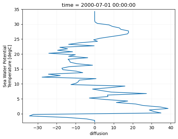
In xwmt, water mass transformations are defined such that they are positive when they tend to increase the mass of water with tracer values less than the given threshold \(\tilde{\lambda}\). For example, \(\mathcal{G}^{(Mix)}(\theta = -1^{\circ}\text{C}) \simeq -35\) Sv means that mixing acts to decrease the mass of water that is colder than -1ºC at a rate of about 35 Sv.

Part 2. Closed and comprehensive water mass transformation budgets

Comprehensive budget dictionary

Using the optional utility package xbudget, we can read in a pre-configured dictionary that contains comprehensive metadata about the structure of tracer budgets in MOM6. (Please feel free to contribute dictionaries for other models!) This dictionary can also be manually created.

import json
import xbudget
print('xbudget version', xbudget.__version__)

budgets_dict = xbudget.load_preset_budget(model="MOM6")
xbudget.collect_budgets(grid, budgets_dict)

print(json.dumps(budgets_dict['heat'], sort_keys=True, indent=4))

xbudget version 0.6.2
{
    "lambda": "thetao",
    "lhs": {
        "sum": {
            "Eulerian_tendency": {
                "product": {
                    "area": "areacello",
                    "tracer_content_tendency_per_unit_area": "opottemptend",
                    "var": "heat_lhs_sum_Eulerian_tendency_product"
                },
                "var": "heat_lhs_sum_Eulerian_tendency"
            },
            "advection": {
                "sum": {
                    "interfacial": {
                        "product": {
                            "area": "areacello",
                            "sign": -1.0,
                            "tracer_content_tendency_per_unit_area": "Th_tendency_vert_remap",
                            "var": "heat_lhs_sum_advection_sum_interfacial_product"
                        },
                        "var": "heat_lhs_sum_advection_sum_interfacial"
                    },
                    "lateral": {
                        "product": {
                            "area": "areacello",
                            "sign": -1.0,
                            "tracer_content_tendency_per_unit_area": "T_advection_xy",
                            "var": "heat_lhs_sum_advection_sum_lateral_product"
                        },
                        "var": "heat_lhs_sum_advection_sum_lateral"
                    },
                    "var": "heat_lhs_sum_advection_sum"
                },
                "var": "heat_lhs_sum_advection"
            },
            "surface_ocean_flux_advective_negative_lhs": {
                "product": {
                    "area": "areacello",
                    "density": 1035.0,
                    "lambda_mass": "tos",
                    "sign": -1.0,
                    "specific_heat_capacity": 3992.0,
                    "thickness_tendency": "boundary_forcing_h_tendency",
                    "var": "heat_lhs_sum_surface_ocean_flux_advective_negative_lhs_product"
                },
                "var": "heat_lhs_sum_surface_ocean_flux_advective_negative_lhs"
            },
            "var": "heat_lhs_sum"
        },
        "var": "heat_lhs"
    },
    "rhs": {
        "sum": {
            "bottom_flux": {
                "product": {
                    "area": "areacello",
                    "tracer_content_tendency_per_unit_area": "internal_heat_heat_tendency",
                    "var": "heat_rhs_sum_bottom_flux_product"
                },
                "var": "heat_rhs_sum_bottom_flux"
            },
            "diffusion": {
                "sum": {
                    "interfacial": {
                        "product": {
                            "area": "areacello",
                            "tracer_content_tendency_per_unit_area": "opottempdiff",
                            "var": "heat_rhs_sum_diffusion_sum_interfacial_product"
                        },
                        "var": "heat_rhs_sum_diffusion_sum_interfacial"
                    },
                    "lateral": {
                        "product": {
                            "area": "areacello",
                            "tracer_content_tendency_per_unit_area": "opottemppmdiff",
                            "var": "heat_rhs_sum_diffusion_sum_lateral_product"
                        },
                        "var": "heat_rhs_sum_diffusion_sum_lateral"
                    },
                    "var": "heat_rhs_sum_diffusion_sum"
                },
                "var": "heat_rhs_sum_diffusion"
            },
            "frazil_ice": {
                "product": {
                    "area": "areacello",
                    "tracer_content_tendency_per_unit_area": "frazil_heat_tendency",
                    "var": "heat_rhs_sum_frazil_ice_product"
                },
                "var": "heat_rhs_sum_frazil_ice"
            },
            "surface_exchange_flux": {
                "product": {
                    "area": "areacello",
                    "tracer_content_tendency_per_unit_area": "boundary_forcing_heat_tendency",
                    "var": "heat_rhs_sum_surface_exchange_flux_product"
                },
                "sum": {
                    "advective": {
                        "product": {
                            "area": "areacello",
                            "tracer_content_tendency_per_unit_area": "heat_content_surfwater",
                            "var": "heat_rhs_sum_surface_exchange_flux_sum_advective_product"
                        },
                        "var": "heat_rhs_sum_surface_exchange_flux_sum_advective"
                    },
                    "nonadvective": {
                        "sum": {
                            "latent": {
                                "product": {
                                    "area": "areacello",
                                    "tracer_content_tendency_per_unit_area": "hflso",
                                    "var": "heat_rhs_sum_surface_exchange_flux_sum_nonadvective_sum_latent_product"
                                },
                                "var": "heat_rhs_sum_surface_exchange_flux_sum_nonadvective_sum_latent"
                            },
                            "longwave": {
                                "product": {
                                    "area": "areacello",
                                    "tracer_content_tendency_per_unit_area": "rlntds",
                                    "var": "heat_rhs_sum_surface_exchange_flux_sum_nonadvective_sum_longwave_product"
                                },
                                "var": "heat_rhs_sum_surface_exchange_flux_sum_nonadvective_sum_longwave"
                            },
                            "sensible": {
                                "product": {
                                    "area": "areacello",
                                    "tracer_content_tendency_per_unit_area": "hfsso",
                                    "var": "heat_rhs_sum_surface_exchange_flux_sum_nonadvective_sum_sensible_product"
                                },
                                "var": "heat_rhs_sum_surface_exchange_flux_sum_nonadvective_sum_sensible"
                            },
                            "shortwave": {
                                "product": {
                                    "area": "areacello",
                                    "tracer_content_tendency_per_unit_area": "rsdoabsorb",
                                    "var": "heat_rhs_sum_surface_exchange_flux_sum_nonadvective_sum_shortwave_product"
                                },
                                "var": "heat_rhs_sum_surface_exchange_flux_sum_nonadvective_sum_shortwave"
                            },
                            "var": "heat_rhs_sum_surface_exchange_flux_sum_nonadvective_sum"
                        },
                        "var": "heat_rhs_sum_surface_exchange_flux_sum_nonadvective"
                    },
                    "var": "heat_rhs_sum_surface_exchange_flux_sum"
                },
                "var": "heat_rhs_sum_surface_exchange_flux"
            },
            "surface_ocean_flux_advective_negative_rhs": {
                "product": {
                    "area": "areacello",
                    "density": 1035.0,
                    "lambda_mass": "tos",
                    "sign": -1.0,
                    "specific_heat_capacity": 3992.0,
                    "thickness_tendency": "boundary_forcing_h_tendency",
                    "var": "heat_rhs_sum_surface_ocean_flux_advective_negative_rhs_product"
                },
                "var": "heat_rhs_sum_surface_ocean_flux_advective_negative_rhs"
            },
            "var": "heat_rhs_sum"
        },
        "var": "heat_rhs"
    },
    "surface_lambda": "tos"
}

Note how this nested dictionary structure allows diagnostics which are unavailable in the convenient layer-integrated form of our example above to be derived or approximated from other available variables. For example, consider the advective surface ocean heat flux, which is described by the sub-dictionary

"surface_ocean_flux_advective_negative_rhs": {
    "product": {
        "area": "areacello",
        "density": 1035.0,
        "lambda_mass": "tos",
        "sign": -1.0,
        "specific_heat_capacity": 3992.0,
        "thickness_tendency": "boundary_forcing_h_tendency",
        "var": "heat_rhs_sum_surface_ocean_flux_advective_negative_rhs_product"
    },

This gives xbudget instructions on how to reconstruct the surface_ocean_flux_advective_negative_rhs tendency as a product of other terms: \begin{equation} -\lambda_{m}Q_{m} \text{d}A = (-1)*(c_{p}*\Theta_{m})*\big(\rho_{0}*\big[\frac{\partial h}{\partial t}\big]_{boundary}\big) * \text{d}A \end{equation}

By calling xbudget.collect_budgets, every derived term in the budget is given a standardized name and lazily added to the dataset grid._ds. For example, the lazily-calculated term described above is stored as:

grid._ds['heat_rhs_sum_surface_ocean_flux_advective_negative_rhs_product']

<xarray.DataArray 'heat_rhs_sum_surface_ocean_flux_advective_negative_rhs_product' (
                                                                                    time: 1,
                                                                                    yh: 180,
                                                                                    xh: 240,
                                                                                    sigma2_l: 74)> Size: 26MB
dask.array<mul, shape=(1, 180, 240, 74), dtype=float64, chunksize=(1, 180, 240, 74), chunktype=numpy.ndarray>
Coordinates:
  * time       (time) object 8B 2000-07-01 00:00:00
  * yh         (yh) int64 1kB 0 1 2 3 4 5 6 7 ... 173 174 175 176 177 178 179
  * xh         (xh) int64 2kB 0 1 2 3 4 5 6 7 ... 233 234 235 236 237 238 239
    areacello  (yh, xh) float64 346kB dask.array<chunksize=(180, 240), meta=np.ndarray>
    deptho     (yh, xh) float32 173kB dask.array<chunksize=(180, 240), meta=np.ndarray>
    geolat     (yh, xh) float64 346kB dask.array<chunksize=(180, 240), meta=np.ndarray>
    geolon     (yh, xh) float64 346kB dask.array<chunksize=(180, 240), meta=np.ndarray>
    lat        (yh, xh) float64 346kB dask.array<chunksize=(180, 240), meta=np.ndarray>
    lon        (yh, xh) float64 346kB dask.array<chunksize=(180, 240), meta=np.ndarray>
    wet        (yh, xh) float32 173kB dask.array<chunksize=(180, 240), meta=np.ndarray>
  * sigma2_l   (sigma2_l) float64 592B 4.246 13.57 17.71 ... 37.76 37.9 38.49
    rho2_l     (sigma2_l) float64 592B dask.array<chunksize=(74,), meta=np.ndarray>
Attributes:
    time_avg_info:  average_T1,average_T2,average_DT
    cell_methods:   area:sum yh:sum xh:sum time: point
    long_name:      Ocean Grid-Cell Area
    note:           We ignore land cells in partially wet cells when coarseni...
    units:          m2
    provenance:     [-1.0, 3992.0, 'tos', 'boundary_forcing_h_tendency', 1035...

xarray.DataArray

'heat_rhs_sum_surface_ocean_flux_advective_negative_rhs_product'

• time: 1
• yh: 180
• xh: 240
• sigma2_l: 74

• dask.array<chunksize=(1, 180, 240, 74), meta=np.ndarray>

  Array Chunk Bytes 24.39 MiB 24.39 MiB Shape (1, 180, 240, 74) (1, 180, 240, 74) Dask graph 1 chunks in 21 graph layers Data type float64 numpy.ndarray

• Coordinates: (12)
  • time
    (time)
    object
    2000-07-01 00:00:00

    axis :

    T

    bounds :

    time_bnds

    calendar_type :

    NOLEAP

    cell_methods :

    time:mean

    long_name :

    historical time

    array([cftime.DatetimeNoLeap(2000, 7, 1, 0, 0, 0, 0, has_year_zero=True)],
          dtype=object)

  • yh
    (yh)
    int64
    0 1 2 3 4 5 ... 175 176 177 178 179

    cell_methods :

    yh:point

    long_name :

    cell center y-index (nominally latitude)

    array([  0,   1,   2,   3,   4,   5,   6,   7,   8,   9,  10,  11,  12,  13,
            14,  15,  16,  17,  18,  19,  20,  21,  22,  23,  24,  25,  26,  27,
            28,  29,  30,  31,  32,  33,  34,  35,  36,  37,  38,  39,  40,  41,
            42,  43,  44,  45,  46,  47,  48,  49,  50,  51,  52,  53,  54,  55,
            56,  57,  58,  59,  60,  61,  62,  63,  64,  65,  66,  67,  68,  69,
            70,  71,  72,  73,  74,  75,  76,  77,  78,  79,  80,  81,  82,  83,
            84,  85,  86,  87,  88,  89,  90,  91,  92,  93,  94,  95,  96,  97,
            98,  99, 100, 101, 102, 103, 104, 105, 106, 107, 108, 109, 110, 111,
           112, 113, 114, 115, 116, 117, 118, 119, 120, 121, 122, 123, 124, 125,
           126, 127, 128, 129, 130, 131, 132, 133, 134, 135, 136, 137, 138, 139,
           140, 141, 142, 143, 144, 145, 146, 147, 148, 149, 150, 151, 152, 153,
           154, 155, 156, 157, 158, 159, 160, 161, 162, 163, 164, 165, 166, 167,
           168, 169, 170, 171, 172, 173, 174, 175, 176, 177, 178, 179])

  • xh
    (xh)
    int64
    0 1 2 3 4 5 ... 235 236 237 238 239

    cell_methods :

    xh:point

    long_name :

    cell center x-index (nominally longitude)

    array([  0,   1,   2, ..., 237, 238, 239], shape=(240,))

  • areacello
    (yh, xh)
    float64
    dask.array<chunksize=(180, 240), meta=np.ndarray>

    cell_methods :

    area:sum yh:sum xh:sum time: point

    long_name :

    Ocean Grid-Cell Area

    note :

    We ignore land cells in partially wet cells when coarsening, so that tracer content can be accurately reconstructed by multiplying coarsened area-averaged tendencies by it. Fully wet (`wet==1.0`) and fully dry (`wet==0.0`) cells should be unaffected, and will just represent the total cell area. For the partially wet cells, total cell area can be derived from the ocean area by divding `areacello` by `wet`.

    standard_name :

    cell_area

    units :

    m2

    Array Chunk Bytes 337.50 kiB 337.50 kiB Shape (180, 240) (180, 240) Dask graph 1 chunks in 2 graph layers Data type float64 numpy.ndarray

  • deptho
    (yh, xh)
    float32
    dask.array<chunksize=(180, 240), meta=np.ndarray>

    cell_measures :

    area: areacello

    cell_methods :

    xh:mean yh:mean time:point

    long_name :

    Sea Floor Depth

    standard_name :

    sea_floor_depth_below_geoid

    units :

    m

    Array Chunk Bytes 168.75 kiB 168.75 kiB Shape (180, 240) (180, 240) Dask graph 1 chunks in 2 graph layers Data type float32 numpy.ndarray

  • geolat
    (yh, xh)
    float64
    dask.array<chunksize=(180, 240), meta=np.ndarray>

    cell_methods :

    time: point

    long_name :

    Latitude of tracer (T) points

    units :

    degrees_north

    Array Chunk Bytes 337.50 kiB 337.50 kiB Shape (180, 240) (180, 240) Dask graph 1 chunks in 2 graph layers Data type float64 numpy.ndarray

  • geolon
    (yh, xh)
    float64
    dask.array<chunksize=(180, 240), meta=np.ndarray>

    cell_methods :

    time: point

    long_name :

    Longitude of tracer (T) points

    units :

    degrees_east

    Array Chunk Bytes 337.50 kiB 337.50 kiB Shape (180, 240) (180, 240) Dask graph 1 chunks in 2 graph layers Data type float64 numpy.ndarray

  • lat
    (yh, xh)
    float64
    dask.array<chunksize=(180, 240), meta=np.ndarray>

    cell_methods :

    time: point

    long_name :

    Latitude of tracer (T) points

    units :

    degrees_north

    Array Chunk Bytes 337.50 kiB 337.50 kiB Shape (180, 240) (180, 240) Dask graph 1 chunks in 2 graph layers Data type float64 numpy.ndarray

  • lon
    (yh, xh)
    float64
    dask.array<chunksize=(180, 240), meta=np.ndarray>

    cell_methods :

    time: point

    long_name :

    Longitude of tracer (T) points

    units :

    degrees_east

    Array Chunk Bytes 337.50 kiB 337.50 kiB Shape (180, 240) (180, 240) Dask graph 1 chunks in 2 graph layers Data type float64 numpy.ndarray

  • wet
    (yh, xh)
    float32
    dask.array<chunksize=(180, 240), meta=np.ndarray>

    cell_measures :

    area: areacello

    cell_methods :

    xh:mean yh:mean time:point

    long_name :

    0 if land, 1 if ocean at tracer points

    note :

    Can be between 0 and 1 if coarse cell includes both wet and dry sub-cells.

    Array Chunk Bytes 168.75 kiB 168.75 kiB Shape (180, 240) (180, 240) Dask graph 1 chunks in 2 graph layers Data type float32 numpy.ndarray

  • sigma2_l
    (sigma2_l)
    float64
    4.246 13.57 17.71 ... 37.9 38.49

    axis :

    Z

    cell_methods :

    sigma2_l:point

    edges :

    sigma2_i

    long_name :

    Target Potential Density minus 1000 kg/m3 at cell center

    positive :

    down

    units :

    kg m-3

    array([ 4.24625, 13.565  , 17.71   , 21.855  , 25.96375, 28.165  , 28.495  ,
           28.83   , 29.165  , 29.495  , 29.83   , 30.165  , 30.495  , 30.83   ,
           31.165  , 31.495  , 31.83   , 32.165  , 32.495  , 32.83   , 33.0665 ,
           33.28225, 33.571  , 33.8425 , 34.09975, 34.3435 , 34.5735 , 34.7895 ,
           34.991  , 35.17725, 35.348  , 35.5035 , 35.64475, 35.77275, 35.8885 ,
           35.99375, 36.09025, 36.17925, 36.262  , 36.34   , 36.4145 , 36.4865 ,
           36.5565 , 36.625  , 36.692  , 36.75525, 36.812  , 36.86125, 36.904  ,
           36.9415 , 36.974  , 37.002  , 37.02625, 37.0475 , 37.0665 , 37.08375,
           37.1    , 37.116  , 37.132  , 37.148  , 37.164  , 37.18   , 37.1965 ,
           37.2145 , 37.235  , 37.26   , 37.2945 , 37.345  , 37.415  , 37.5075 ,
           37.625  , 37.76   , 37.9    , 38.485  ])

  • rho2_l
    (sigma2_l)
    float64
    dask.array<chunksize=(74,), meta=np.ndarray>

    axis :

    Z

    edges :

    rho2_i

    long_name :

    Target Potential Density at cell center

    positive :

    down

    units :

    kg m-3

    Array Chunk Bytes 592 B 592 B Shape (74,) (74,) Dask graph 1 chunks in 2 graph layers Data type float64 numpy.ndarray

• Attributes: (6)

  time_avg_info :

  average_T1,average_T2,average_DT

  cell_methods :

  area:sum yh:sum xh:sum time: point

  long_name :

  Ocean Grid-Cell Area

  note :

  We ignore land cells in partially wet cells when coarsening, so that tracer content can be accurately reconstructed by multiplying coarsened area-averaged tendencies by it. Fully wet (`wet==1.0`) and fully dry (`wet==0.0`) cells should be unaffected, and will just represent the total cell area. For the partially wet cells, total cell area can be derived from the ocean area by divding `areacello` by `wet`.

  units :

  m2

  provenance :

  [-1.0, 3992.0, 'tos', 'boundary_forcing_h_tendency', 1035.0, 'areacello']

The full dictionary is daunting, but we don’t need every term just to close the water mass transformation budget. We can use the xbudget.aggregate function to just pick out the highest-level terms in the budget.

simple_budgets = xbudget.aggregate(budgets_dict)
print(json.dumps(simple_budgets, sort_keys=True, indent=4))

{
    "heat": {
        "lambda": "thetao",
        "lhs": {
            "Eulerian_tendency": "heat_lhs_sum_Eulerian_tendency",
            "advection": "heat_lhs_sum_advection",
            "surface_ocean_flux_advective_negative_lhs": "heat_lhs_sum_surface_ocean_flux_advective_negative_lhs"
        },
        "rhs": {
            "bottom_flux": "heat_rhs_sum_bottom_flux",
            "diffusion": "heat_rhs_sum_diffusion",
            "frazil_ice": "heat_rhs_sum_frazil_ice",
            "surface_exchange_flux": "heat_rhs_sum_surface_exchange_flux",
            "surface_ocean_flux_advective_negative_rhs": "heat_rhs_sum_surface_ocean_flux_advective_negative_rhs"
        },
        "surface_lambda": "tos"
    },
    "mass": {
        "lambda": "density",
        "lhs": {
            "Eulerian_tendency": "mass_lhs_sum_Eulerian_tendency"
        },
        "rhs": {
            "advection": "mass_rhs_sum_advection",
            "surface_exchange_flux": "mass_rhs_sum_surface_exchange_flux"
        },
        "thickness": "thkcello"
    },
    "salt": {
        "lambda": "so",
        "lhs": {
            "Eulerian_tendency": "salt_lhs_sum_Eulerian_tendency",
            "advection": "salt_lhs_sum_advection",
            "surface_ocean_flux_advective_negative_lhs": "salt_lhs_sum_surface_ocean_flux_advective_negative_lhs"
        },
        "rhs": {
            "diffusion": "salt_rhs_sum_diffusion",
            "surface_exchange_flux": "salt_rhs_sum_surface_exchange_flux",
            "surface_ocean_flux_advective_negative_rhs": "salt_rhs_sum_surface_ocean_flux_advective_negative_rhs"
        },
        "surface_lambda": "sos"
    }
}

Redundancy of derived terms

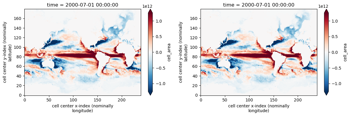
Some terms in the budget, such as the water mass transformation due to surface heat fluxes, can be equivalently derived from two different sets of budget diagnostics:

term = budgets_dict['heat']['rhs']['sum']['surface_exchange_flux']
print("As the product of the layer-integrated convergence of surface heat fluxes, multiplied with the cell area:")
print(json.dumps(term['product'], sort_keys=True, indent=4), end="\n\n")
print("Or as the sum of the individual heat surface heat fluxes\n(where we distinguish advection and non-advective contributions),\neach individually multiplied by the cell area:")
print(json.dumps(term['sum'], sort_keys=True, indent=4))

As the product of the layer-integrated convergence of surface heat fluxes, multiplied with the cell area:
{
    "area": "areacello",
    "tracer_content_tendency_per_unit_area": "boundary_forcing_heat_tendency",
    "var": "heat_rhs_sum_surface_exchange_flux_product"
}

Or as the sum of the individual heat surface heat fluxes
(where we distinguish advection and non-advective contributions),
each individually multiplied by the cell area:
{
    "advective": {
        "product": {
            "area": "areacello",
            "tracer_content_tendency_per_unit_area": "heat_content_surfwater",
            "var": "heat_rhs_sum_surface_exchange_flux_sum_advective_product"
        },
        "var": "heat_rhs_sum_surface_exchange_flux_sum_advective"
    },
    "nonadvective": {
        "sum": {
            "latent": {
                "product": {
                    "area": "areacello",
                    "tracer_content_tendency_per_unit_area": "hflso",
                    "var": "heat_rhs_sum_surface_exchange_flux_sum_nonadvective_sum_latent_product"
                },
                "var": "heat_rhs_sum_surface_exchange_flux_sum_nonadvective_sum_latent"
            },
            "longwave": {
                "product": {
                    "area": "areacello",
                    "tracer_content_tendency_per_unit_area": "rlntds",
                    "var": "heat_rhs_sum_surface_exchange_flux_sum_nonadvective_sum_longwave_product"
                },
                "var": "heat_rhs_sum_surface_exchange_flux_sum_nonadvective_sum_longwave"
            },
            "sensible": {
                "product": {
                    "area": "areacello",
                    "tracer_content_tendency_per_unit_area": "hfsso",
                    "var": "heat_rhs_sum_surface_exchange_flux_sum_nonadvective_sum_sensible_product"
                },
                "var": "heat_rhs_sum_surface_exchange_flux_sum_nonadvective_sum_sensible"
            },
            "shortwave": {
                "product": {
                    "area": "areacello",
                    "tracer_content_tendency_per_unit_area": "rsdoabsorb",
                    "var": "heat_rhs_sum_surface_exchange_flux_sum_nonadvective_sum_shortwave_product"
                },
                "var": "heat_rhs_sum_surface_exchange_flux_sum_nonadvective_sum_shortwave"
            },
            "var": "heat_rhs_sum_surface_exchange_flux_sum_nonadvective_sum"
        },
        "var": "heat_rhs_sum_surface_exchange_flux_sum_nonadvective"
    },
    "var": "heat_rhs_sum_surface_exchange_flux_sum"
}

We can plot these to verify that they are indeed equivalent (to machine precision):

plt.figure(figsize=(12, 4))
plt.subplot(1,2,1)
grid._ds[term['product']['var']].sum("sigma2_l").plot(robust=True)
plt.subplot(1,2,2)
grid._ds[term['sum']['var']].sum("sigma2_l").plot(robust=True)
plt.tight_layout()

Compute water mass transformations

Finally, we can create an instance of the core WaterMassTransformations class and verify that it can find all of the processes we need in the dataset.

wmt = xwmt.WaterMassTransformations(grid, simple_budgets)
sorted(wmt.available_processes())

['Eulerian_tendency',
 'advection',
 'bottom_flux',
 'diffusion',
 'frazil_ice',
 'surface_exchange_flux',
 'surface_ocean_flux_advective_negative_lhs',
 'surface_ocean_flux_advective_negative_rhs']

We use the integrate_transformations method to compute area-integrated water mass transformations in the specified coordinate (e.g. "heat").

import warnings
with warnings.catch_warnings():
    warnings.simplefilter(action='ignore', category=FutureWarning)

    kwargs = {"sum_components":True, "group_processes":True}
    G_temperature = wmt.integrate_transformations(
        "heat",
        bins=np.arange(-3, 35, 0.25),
        **kwargs
    ).mean('time')
    G_salinity = wmt.integrate_transformations(
        "salt",
        bins=np.arange(0, 50, 0.25),
        **kwargs
    ).mean('time')
    G_density = wmt.integrate_transformations(
        "sigma0",
        bins=np.arange(0, 40, 0.25),
        **kwargs
    ).mean('time')

Gs = [G_temperature, G_salinity, G_density]

Process 'bottom_flux' for component salt is unavailable.
Process 'frazil_ice' for component salt is unavailable.

for G in Gs:
    with ProgressBar():
        G.load()

[########################################] | 100% Completed | 407.05 ms
[########################################] | 100% Completed | 406.28 ms
[########################################] | 100% Completed | 835.86 ms

Finally, we can plot the WMT associated with each of the terms and verify that our water mass transformation budgets close:

long_names =  [r"potential temperature [$\degree$C]", r"practical salinity [psu]", r"potential density $\sigma_{0}$ [kg/m$^{3}$-1000]"]

plt.figure(figsize=(12, 9))
for i, (G, long_name) in enumerate(zip(Gs, long_names)):
    plt.subplot(3,1,i+1)
    for v in sorted(wmt.available_processes()):
        if v not in G: continue
        G[v].plot(label=v)
    G['kinematic_transformation'].plot(label="Kinematic WMT (LHS)", color="k")
    G['material_transformation'].plot(label="Process-based WMT (RHS)", ls="--", color="grey")
    plt.legend(loc=(1.03, 0.))
    plt.ylabel("WMT rate [kg/s]")
    plt.xlabel(long_name)
    plt.grid(True, alpha=0.15)
plt.tight_layout()

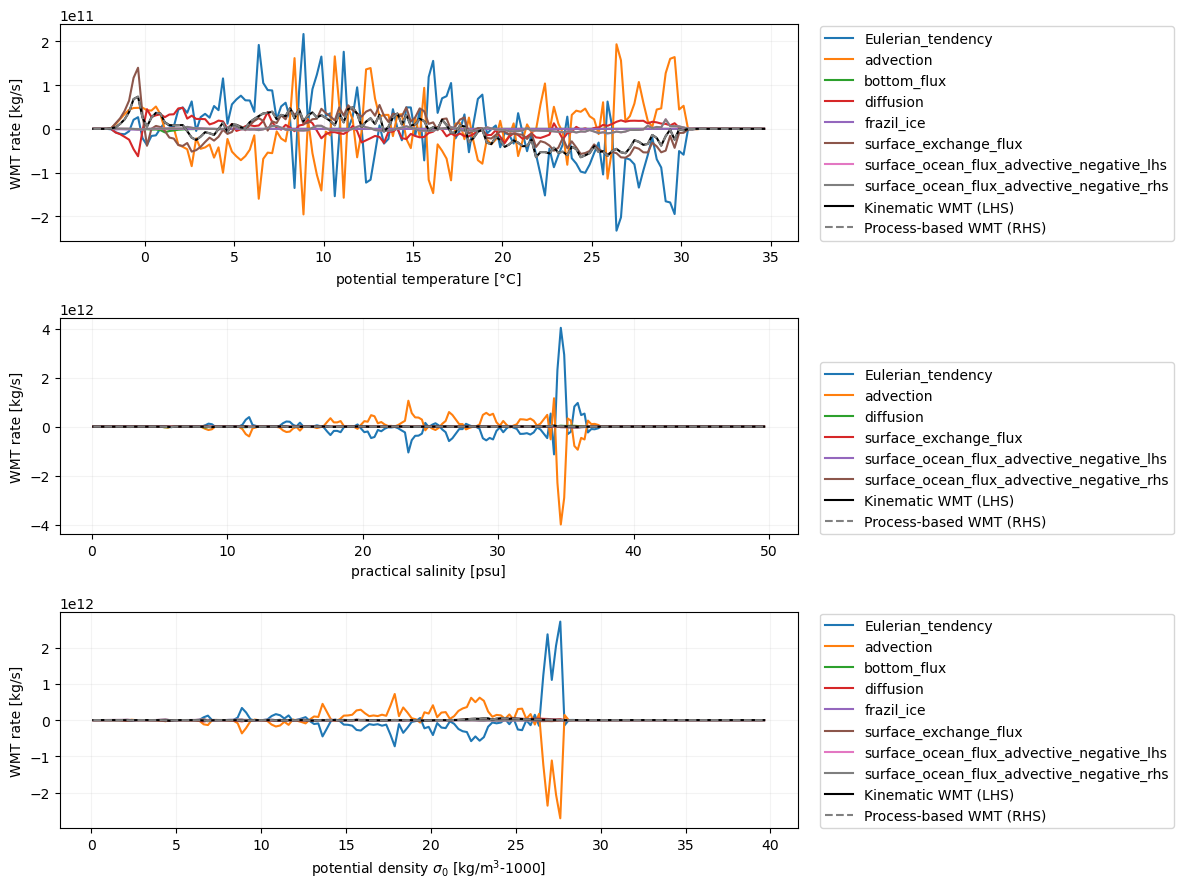
We see that there is a high degree of cancellation between two of the terms on the LHS of the transformation equation: the tendency term and the advection term. In water mass transformation, theory, however, we are more interested in the transformation terms that appear on the RHS of the equation.

Part 3. Selectively decomposing budget terms

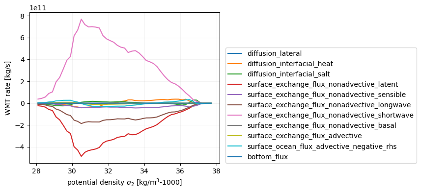
In density coordinates, there seems to be a dominant balance between the diffusive and surface fluxes terms on the RHS.

Let’s break those processes down even further to gain a better understanding.

decomposed_budgets = xbudget.aggregate(budgets_dict, decompose=["diffusion", "surface_exchange_flux", "nonadvective"])
wmt = xwmt.WaterMassTransformations(grid, decomposed_budgets)
import warnings
with warnings.catch_warnings():
    warnings.simplefilter(action='ignore', category=FutureWarning)

    G_density = wmt.integrate_transformations(
        "sigma2",
        bins=np.arange(28, 38, 0.2),
        **kwargs
    ).mean('time')
    with ProgressBar():
        G_density.load()

[########################################] | 100% Completed | 815.55 ms

G = G_density
long_name = r"potential density $\sigma_{2}$ [kg/m$^{3}$-1000]"

processes = [
    "diffusion_lateral",
    "diffusion_interfacial_heat",
    "diffusion_interfacial_salt",
    "surface_exchange_flux_nonadvective_latent",
    "surface_exchange_flux_nonadvective_sensible",
    "surface_exchange_flux_nonadvective_longwave",
    "surface_exchange_flux_nonadvective_shortwave",
    "surface_exchange_flux_nonadvective_basal",
    "surface_exchange_flux_advective",
    "surface_ocean_flux_advective_negative_rhs",
    "frazil_heat_tendency",
    "bottom_flux",
]

plt.figure(figsize=(5, 4))
for v in processes:
    if v not in G: continue
    G[v].plot(label=v)
plt.legend(loc=(1.03, 0))
plt.ylabel("WMT rate [kg/s]")
plt.xlabel(long_name)
plt.grid(True, alpha=0.15)

Part 4: Mapping spatial patterns of water mass transformation

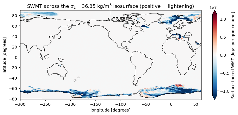
Suppose we are interested in better understanding how surface exchange fluxes drive the formation of dense waters and where these transformations occur spatially.

Instead of integrate_transformations, we can use map_transformations to compute the transformation in each grid columns.

sigma2_lev = 36.85

wmt = xwmt.WaterMassTransformations(grid, simple_budgets)

with warnings.catch_warnings():
    warnings.simplefilter(action='ignore', category=FutureWarning)
    G_density_map = (
        wmt.map_transformations("sigma2", bins=np.arange(28, 38, 0.2))
        .sel(sigma2_l_target=sigma2_lev, method="nearest")
    );
    with ProgressBar():
        G_density_map.load();

[########################################] | 100% Completed | 810.00 ms

total_surface_forced_flux = (
    G_density_map["surface_exchange_flux"] + # part due to direct fluxes of heat and salt
    G_density_map["surface_ocean_flux_advective_negative_rhs"] # part due to freshwater fluxes that dilute/concentrate salt and temperature
)

plt.figure(figsize=(10, 4))
pc = total_surface_forced_flux.plot(x="geolon", y="geolat", robust=True)
(G_density_map.wet == 0).plot.contour(levels=[0], colors="k", x="geolon", y="geolat", linewidths=0.75)
plt.title("");
plt.xlabel("longitude [degrees]")
plt.ylabel("latitude [degrees]")
pc.colorbar.set_label("Surface-forced WMT [kg/s per grid column]")
plt.title(rf"SWMT across the $\sigma_{{2}} = {sigma2_lev}$ kg/m$^{{3}}$ isosurface (positive = lightening)");